This note concerns my take on the derivation of the vector equations for a standard ray tracing diagram ubiquitous in geometric optics and computer graphics. The diagram is appropriate for a ray incident on a point on a locally flat interface between two material regions. For non-normal incidence, the vectors of interest lie in the incident plane formed by the ray and the surface normal at the point of incidence. The vector equations are well-known, but we include them as a necessary mathematical tool and starting point for further computational tools and results.
The standard ray tracing diagram is illustrated below.
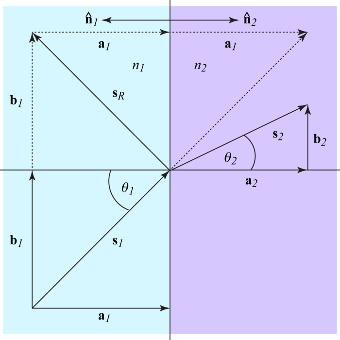
Geometric quantities and material properties are indexed with a subscript indicating the “from” medium having index 1 or the “to” medium having index 2. Definitions for the quantities illustrated in the ray tracing diagram are defined in the table below

Note that the incident and transmitted normal angles must lie between zero and 

The incident cosine vector can thus be written as

Two vector sums can be inferred directly from the figure

Solving for 


It can likewise be shown that

and we write

Note that this representation for the reflected ray is invariant under the transformation 
Computation of the transmitted direction requires Snell’s law

Since the incident and transmitted vectors are unit vectors it follows that

The sine vectors for the incident and transmitted rays have different magnitudes but point in the same direction


It is therefore possible to write the sine vector for the transmitted direction as

where the parameter 
Total internal reflection, or TIR, occurs when

Based on the ray tracing diagram, it is straightforward to write the vector sum

Putting this in the TIR inequality test above gives

This requires no computation of trigonometric functions or square roots. If the index ratio is pre-computed then the TIR test also requires no division operations.
From the ray tracing diagram, the cosine vector for the incident ray can be written as

The cosine vector for the transmitted ray points in the same direction as the incident ray but has a different magnitude

where 

Noting that the incident and transmitted angles must be on the interval ![\displaystyle \left[ {0,{\pi }/{2}\;} \right]](https://s0.wp.com/latex.php?latex=%5Cdisplaystyle+%5Cleft%5B+%7B0%2C%7B%5Cpi+%7D%2F%7B2%7D%5C%3B%7D+%5Cright%5D&bg=f5f6f7&fg=444444&s=0&c=20201002)

Putting this together, the transmitted ray is
![\displaystyle {{\mathbf{s}}_{2}}={{\mathbf{a}}_{2}}+{{\mathbf{b}}_{2}}=\mathbf{\hat{n}}\ \text{sgn} \left( {{{\mathbf{s}}_{1}}\cdot \mathbf{\hat{n}}} \right)\sqrt{{1-N_{R}^{2}{{{\left| {{{\mathbf{s}}_{1}}-\mathbf{\hat{n}}\left( {{{\mathbf{s}}_{1}}\cdot \mathbf{\hat{n}}} \right)} \right|}}^{2}}}}+{{N}_{R}}\left[ {{{\mathbf{s}}_{1}}-\mathbf{\hat{n}}\left( {{{\mathbf{s}}_{1}}\cdot \mathbf{\hat{n}}} \right)} \right]](https://s0.wp.com/latex.php?latex=%5Cdisplaystyle+%7B%7B%5Cmathbf%7Bs%7D%7D_%7B2%7D%7D%3D%7B%7B%5Cmathbf%7Ba%7D%7D_%7B2%7D%7D%2B%7B%7B%5Cmathbf%7Bb%7D%7D_%7B2%7D%7D%3D%5Cmathbf%7B%5Chat%7Bn%7D%7D%5C+%5Ctext%7Bsgn%7D+%5Cleft%28+%7B%7B%7B%5Cmathbf%7Bs%7D%7D_%7B1%7D%7D%5Ccdot+%5Cmathbf%7B%5Chat%7Bn%7D%7D%7D+%5Cright%29%5Csqrt%7B%7B1-N_%7BR%7D%5E%7B2%7D%7B%7B%7B%5Cleft%7C+%7B%7B%7B%5Cmathbf%7Bs%7D%7D_%7B1%7D%7D-%5Cmathbf%7B%5Chat%7Bn%7D%7D%5Cleft%28+%7B%7B%7B%5Cmathbf%7Bs%7D%7D_%7B1%7D%7D%5Ccdot+%5Cmathbf%7B%5Chat%7Bn%7D%7D%7D+%5Cright%29%7D+%5Cright%7C%7D%7D%5E%7B2%7D%7D%7D%7D%2B%7B%7BN%7D_%7BR%7D%7D%5Cleft%5B+%7B%7B%7B%5Cmathbf%7Bs%7D%7D_%7B1%7D%7D-%5Cmathbf%7B%5Chat%7Bn%7D%7D%5Cleft%28+%7B%7B%7B%5Cmathbf%7Bs%7D%7D_%7B1%7D%7D%5Ccdot+%5Cmathbf%7B%5Chat%7Bn%7D%7D%7D+%5Cright%29%7D+%5Cright%5D&bg=f5f6f7&fg=444444&s=0&c=20201002)
It is easy to see that the representation for the transmitted ray is invariant under the transformation

Looks great Tom. I’m looking forward to seeing more of your work.
LikeLike
Thank you, Keith!
LikeLike
Congrats on the birth of Mathammer.com!
LikeLike
Thank you, Bryan! It is a start 🙂
LikeLike